rational agent should select an action that is expected
to maximize its performance measure, given the
evidence provided by the percept sequence and
whatever built-in knowledge the agent has.
Setting for intelligent design:
PEAS: Performance measure (safest), Environment (road), Actuators (horn, brake),
Sensors (speedometer, camera)
A problem is defined by four items:
1. initial state (Arad)
2. actions or successor functions (Arad->Zenrind)
3. goal test (Bucharest)
4. path cost (# of actions executed, nodes visited)
tree search - expanding states / nodes
completeness: does it always find a solution if one exists?
time complexity: number of nodes generated
space complexity: maximum number of nodes in memory
optimality: does it always find a least-cost solution?
uninformed search:
- breadth-first - fifo, go wide, time and space = O(b^d+1),
- depth-first - lifo, go deep, time=O(b^m), space = O(bm) (only keep one path in memory)
- depth limited
- iterative-deepening
Uninformed search - Summary
• Problem formulation usually requires abstracting away real-
world details to define a state space that can feasibly be
explored
•
• Variety of uninformed search strategies
•
• Iterative deepening search uses only linear space and not
much more time than other uninformed algorithms
•
A*
Evaluation function f(n) = g(n) + h(n)
g(n) = cost so far to reach n
h(n) = estimated cost from n to goal
f(n) = estimated total cost of path through n to
goal
Theorem: If h(n) is admissible, A* using TREE-
SEARCH is optimal
Local search:
- hill-climbing (climb mount everest in thick fog with amnesia)
- simulated annealing (allow bad moves but decrease their frequency)
- local beam search
- genetic algorithms
Informed-Search Summary
• Heuristic functions estimate costs of shortest paths
• Good heuristics can dramatically reduce search cost
• Greedy best-first search expands lowest h
– – incomplete and not always optimal
• A∗ search expands lowest g + h
– – complete and optimal
– – also optimally efficient (up to tie-breaks, for forward
search)
• Admissible heuristics can be derived from exact
solution of relaxed problems
• Admissible heuristics never overestimates true cost of the solution
constraint satisfaction problem (CSP)
- map-coloring
- nodes are variables
- edges are constraints
back-tracking search is uninformed depth-first search for CSPs
forward checking keeps track of valid legal moves, terminate when there's no more valid moves
arc consistency - An Arc X->Y is consistent if for every value x of X there is some value y in Y consistent with x
if a constraint graph has no loops, then CSP can be solved in O(nd^2) time
- linear in the number of variables.
2 general approaches to convert cyclic graphs to trees
1. Assign values to specific variables (Cycle Cutset method)
2. Construct a tree-decomposition of the graph
- Connected subproblems (subgraphs) form a tree structure
A CSP is k-consistent if for any set of k-1 variables and for any consistent
assignment to those variables, a consistent value can always be assigned to any kth
variable.
solve tree csps by
1. convert graph to tree, pick a parent, so any node only has one parent
2. apply backward pass (constraint propagation)
3. forward pass (assignment)
heuristics:
- Most constrained variable (highest number of edges): choose the variable (eg. SA map) with the fewest legal values
- Least constraining value - Given a variable, choose the least constraining value (eg. pick red)
Arc-consistency (AC) is a systematic procedure for constraining propagation
min-conflict heuristic for hill climbing in n-queens
CSP-Summary
• CSPs
– special kind of problem: states defined by values of a fixed set of variables, goal test
defined by constraints on variable values
• Backtracking=depth-first search with one variable assigned per node
• Heuristics
– Variable ordering and value selection heuristics help significantly
• Constraint propagation does additional work to constrain values and detect
inconsistencies
– Works effectively when combined with heuristics
• Iterative min-conflicts is often effective in practice.
• Graph structure of CSPs determines problem complexity
– e.g., tree structured CSPs can be solved in linear time.
Minimax strategy
Find the optimal strategy for MAX assuming an infallible MIN
opponent
– Need to compute this all the down the tree
alpha-beta pruning
Depth first search – only considers nodes along a single path
at any time
The Horizon Effect
– sometimes there’s a major “effect” (such as a piece being
captured) which is just “below” the depth to which the tree has
been expanded
Expected Minimax = sum_over_chance_nodes(prob(x)+minimax(x))
Minimax - Summary
• Game playing can be effectively modeled as a search problem
• Game trees represent alternate computer/opponent moves
• Evaluation functions estimate the quality of a given board
configuration for the Max player.
• Minimax is a procedure which chooses moves by assuming that
the opponent will always choose the move which is best for
them
• Alpha-Beta is a procedure which can prune large parts of the
search tree and allow search to go deeper
• For many well-known games, computer algorithms based on
heuristic search match or out-perform human world experts.
logic:
m is a model of a sentence alpha if alpha is true in m
alpha |= b, alpha entails sentence b if and only if b is true in all worlds where
alpha is true.
Model-checking enumerates all possible worlds
If an algorithm only derives entailed sentences it is called
sound or truth preserving.
Completeness : the algorithm can derive any sentence that is
entailed.
truth table connectives

Two sentences are logically equivalent iff they are true in same models: α ≡ ß
iff α╞ β and β╞ α
Logical equivalence

A sentence is valid if it is true in all models,
e.g., True, A V ~A, A => A, (A ^ (A => B)) => B
(tautologies)
Validity is connected to inference via the Deduction Theorem:
KB ╞ α if and only if (KB => α) is valid
A sentence is satisfiable if it is true in some model
e.g., A V B, C
(determining satisfiability of sentences is NP-complete)
A sentence is unsatisfiable if it is false in all models
e.g., A ^ ~A
Satisfiability is connected to inference via the following (aka proof by contradiction):
KB ╞ α if and only if (KB ^ ~α) is unsatisfiable
Normal form = conjunctions of disjunctions
Horn clause = A clause with at most 1 positive literal. e.g. A V ~B V ~C = B ^ C => A
1 positive literal: definite clause
Forward chaining (sound and complete for Horn KB)
Idea: fire any rule whose premises are satisfied in the KB,
– add its conclusion to the KB, until query is found
Backward chaining (BC)
check if q is known already, or
prove by BC all premises of some rule concluding q
Hence BC maintains a stack of sub-goals that need to
be proved to get to q.
- Like FC, is linear and is also sound and complete (for Horn KB)
• FC is data-driven, automatic, unconscious processing,
– e.g., object recognition, routine decisions
• May do lots of work that is irrelevant to the goal
• BC is goal-driven, appropriate for problem-solving,
– e.g., Where are my keys? How do I get into a PhD program?
• Complexity of BC can be much less than linear in size of KB
Model Checking (Satisfiability - SAT problems)
Two families of efficient algorithms:
• Complete backtracking search algorithms: DPLL algorithm
• Incomplete local search algorithms
– WalkSAT algorithm (random flipping, only good if we know a solution exists)
Logic - Summary
• Logical agents apply inference to a knowledge base to
derive new information and make decisions
• Basic concepts of logic:
– syntax: formal structure of sentences
– semantics: truth of sentences wrt models
– entailment: necessary truth of one sentence given another
– inference: deriving sentences from other sentences
– soundness: derivations produce only entailed sentences
– completeness: derivations can produce all entailed
sentences
• Resolution is complete for propositional logic
• Forward, backward chaining are linear-time, complete
for Horn clauses
• Propositional logic lacks expressive power
• Propositional logic assumes the world contains facts,
• First-order logic (like natural language) assumes the world
contains
– Objects: people, houses, numbers, colors, baseball games, wars,
...
– Relations (returns True or False - Facts / atomic sentence): Brother(Richard, John)
– Functions (returns another object): LeftLegOf(John), Sqrt(3)
– Variables x, y, a, b,...
– Connectives , , , ,
– Equality =
– Quantifiers ,
Note: Functions do not state facts and form no sentence:
– Brother(Pete) refers to John (his brother) and is neither true nor false.
for all Vx King(x) => Person(x)
there exists Ei Integer(i) ^ GreaterThan(i,0)
Squares are breezy near a pit:
– Diagnostic rule --infer cause (pit / cavity) from effect (breeze / toothache), given a breeze, what's the chances of a pit?
s Breezy(s) r Adjacent(r,s) Pit(r)
– Causal rule---infer effect from cause (model based reasoning), given a pit, what's the chances of a breeze?
r Pit(r) [ s Adjacent(r,s) Breezy(s)]
First-order logic Summary:
– Much more expressive than propositional logic
– Allows objects and relations as semantic primitives
– Universal and existential quantifiers
– syntax: constants, functions, predicates, equality, quantifiers
–
• Knowledge engineering using FOL
– Capturing domain knowledge in logical form
propositionalization (convert FOL to propositional form, problem is generates lots of irrelevant sentences, fix is to use unification):
- Universal instantiation (UI) : Subst({v/g}, α) means the result of substituting ground term g for variable v in sentence α, produces a whole set of instantiated sentences
e.g King(John) Greedy(John) Evil(John), {x/John}
- Existential instantiation (EI) : For any sentence α, variable v, and constant symbol k (that
does not appear elsewhere in the knowledge base):
E.g., x Crown(x) OnHead(x,John) yields:
Crown(C1) OnHead(C1,John)
where C1 is a new constant symbol, called a Skolem constant
Idea for doing inference in FOL:
– propositionalize KB and query
– apply resolution-based inference
– return result
Unification (better way to propositionalize than instantiation):
• Recall: Subst(θ, p) = result of substituting θ into sentence p
• Unify algorithm: takes 2 sentences p and q and returns a
unifier θ if one exists
Unify(p,q) = θ where Subst(θ, p) = Subst(θ, q)
• There is a single most general unifier (MGU) that is unique up
to renaming of variables.
eg. Knows(John,x) and Knows(y,z) MGU θ = { y/John, x/z }
Knows(x,OJ) and Knows(John,x) {fail}!!! because x can't be both OJ and John, fix is to standardize variable (rename x to z so Knows(z,OJ) and Knows(Jonh,x) )
Modus ponens: p, p->q
-------
q
Generalized Modus Ponens (GMP) (slide 13)
p1', p2', ... , pn', ( p1 ^ p2 ^ ... ^ pn -> q)
------------------------------------------------
Subst(θ,q)
where we can unify pi', and pi for all i
Example:
p1' is King(John) p1 is King(x)
p2' is Greedy(y) p2 is Greedy(x)
θ is {x/John,y/John} q is Evil(x)
Subst(θ,q) is Evil(John)
GMP is complete for a KB consisting of definite clauses ( a ^ b -> c = not a V not b or c , 1 positive literal)
• Forward-chaining
– Uses GMP to add new atomic sentences
– Useful for systems that make inferences as information streams in
– Requires KB to be in form of first-order definite clauses
• Backward-chaining
– Works backwards from a query to try to construct a proof
– Can suffer from repeated states and incompleteness
– Useful for query-driven inference
• Resolution-based inference (FOL)
– Refutation-complete for general KB
• Can be used to confirm or refute a sentence p (but not to
generate all entailed sentences)
– Requires FOL KB to be reduced to CNF
– Uses generalized version of propositional inference rule
Prolog
• Closed-world assumption ("negation as failure")
– e.g., given alive(X) :- not dead(X).
– alive(joe) succeeds if dead(joe) fails // so assume joe is alive if he's not dead
Program = set of clauses = head :- literal1, ... literaln.
criminal(X) :- american(X), weapon(Y), sells(X,Y,Z), hostile(Z).
Appending two lists to produce a third:
append([],Y,Y).
append([X|L],Y,[X|Z]) :- append(L,Y,Z).
append(input1, input2, output)
• append(A,B,[1,2]) ? // what input value combinations for A and B will give [1,2] output?
• answers: A=[] B=[1,2]
A=[1] B=[2]
A=[1,2] B=[]
Resolution:
(A V B V C), ~A
-----------------
(B V C)
(A V B V C), ( ~A V D V E)
--------------------------
(B V C V D V E)
FOL inference Summary
• Inference in FOL
– Simple approach: reduce all sentences to PL and apply
propositional inference techniques
– Generally inefficient
• FOL inference techniques
– Unification
– Generalized Modus Ponens
• Forward-chaining: complete with definite clauses
– Resolution-based inference
• Refutation-complete
Eliminate existential quantifiers (Skolemize):
∃x P(x) becomes P(K) (EE)
K is some new constant (Skolem constant)
∀x∃y P(x,y) becomes ∀x P(x,F(x))
F() must be a new function (Skolem function)
Probabilistic assertions summarize effects of
– Laziness - failure to enumerate exceptions, qualifications, etc
– Ignorance - lack of relevant facts, initial conditions, etc.
Default or nonmonotonic logic:
– Assume my car does not have a flat tire
Utility theory is used to represent and infer preferences
Decision theory = probability theory + utility theory
The fundamental idea of decision theory is that an agent is rational if
and only if it chooses the action that yields that highest expected
utility, averaged over all the possible outcomes of the action.
Atomic event: A complete specification of the
state of the world about which the agent is
uncertain
E.g., if the world consists of only two Boolean variables
Cavity and Toothache, then there are 4 distinct
atomic events:
Cavity = false Toothache = false
Cavity = false Toothache = true
Cavity = true Toothache = false
Cavity = true Toothache = true
Axioms of probability
• For any propositions A, B
• 0 ≤ P(A) ≤ 1
– P(true) = 1 and P(false) = 0
– P(A V B) = P(A) + P(B) - P(A ^ B)
In the study of probability, given two random variables X and Y defined on the same probability space, the joint distribution for X and Y defines the probability of events defined in terms of both X and Y
unconditional / prior probability P(A) : probability A will appear in the absence of any other information, eg. P(Cavity) = 0.1
conditional / posterior probability P(A|B) : probability of A changes with respect to new information B eg. P(Cavity|Toothache) = 0.8
P(A|B) = P(A^B)/P(B) can be rewritten as product rule: P(A^B)=P(A|B)P(B)=P(B|A)P(A)
if A and B are independent, then P(A|B)=P(A) so P(A^B)=P(A|B)P(B)=P(A)P(B)
Finetti (2 player game, player1 has subjective probability 'a' on the occurrence of 'b'):
- subjective beliefs should respect the axioms
- If the beliefs are contradictory, then the agent will fail in its environment
in the long run!
- if bet $0.4 for b and P(b)=0.4, if b happens (0.4 chance), we take other player's money who bet $0.6 so 0.4*0.6 and if b doesn't happen (0.6 chance), we loose $0.4 so -0.6*$0.4 so
0.4*$0.6 - 0.6*$0.4 = 0
- so we either pay how much we bet, or win the bet of the other player
Cavity, Toothache, Catch Joint probability distribution
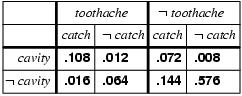
P(toothache) = 0.108 + 0.012 + 0.016 + 0.064 = 0.2
P(toothache or cavity) = P(toothache) + P(cavity) - P(toothache and cavity) = (0.108 + 0.012 + 0.016 + 0.064) + (0.108 + 0.012 + 0.072 + 0.008) - (0.108 + 0.012) = 0.28
P( ~cavity | toothache) = P( ~cavity ^ toothache) / P(toothache)
= (0.016+0.064) / (0.108 + 0.012 + 0.016 + 0.064)
= 0.08 / 0.2 = 0.4
P( cavity | toothache) = P( cavity ^ toothache) / P(toothache)
= (0.108+0.012) / (0.108 + 0.012 + 0.016 + 0.064)
= 0.120 / 0.2 = 0.6
General idea: compute distribution (X) on query variable (Y) by fixing evidence
variables (E) and summing (adding all possible combinations) over hidden variables (H), so H = X - Y - E
• Obvious problems (fix is independence!, divide and conquer):
1. Worst-case time complexity O(dn) where d is the largest arity
2. Space complexity O(dn) to store the joint distribution
3. How to find the numbers for O(dn) entries?
Normalization / Relative likelihood:
let alpha = 1 / P(toothache), hidden variable catch, then
P( cavity | toothache) = alpha * P( cavity ^ toothache) = alpha * P(cavity,toothache,catch) + P(cavity,toothache,~catch) = alpha * (0.108+0.012) = alpha * 0.12
**note, when alpha is involved, need to normalize the final value and to do this, need to find out both P(a) and P(~a) so alpha = 1/(p(a) + p(~a))
Similarly,
P( ~cavity | toothache) = alpha * P( ~cavity ^ toothache) = alpha * P(~cavity,toothache,catch) + P(~cavity,toothache,~catch) = alpha * (0.016+0.064) = alpha * 0.08
To get real probability values,
P(cavity|toothache) + P(~cavity|toothache) = 1
alpha * (0.12+0.08) = 1, alpha = 5, so
P(cavity|toothache) = 5*0.12 = 0.6
P(cavity|toothache) = 5*0.08 = 0.4
Independence: P(Toothache, Catch, Cavity, Weather) = P(Toothache, Catch, Cavity) P(Weather)
So instead of 2*2*2*4=32 entries, it's broken down to 2*2*2+4=12 entries
Catch is conditionally independent of Toothache given Cavity:
• P(Catch | Toothache,Cavity) = P(Catch | Cavity)
So the probe catching it isn't affected by whether or not we have a toothache,
Baye's rule for multiple evidence (toothache, catch) (assuming catch is conditionally independent of toothache given cavity) is:
P(toothache, Cavity, Catch) = alpha * P(toothache|cavity) * P(catch|cavity) * P(cavity)
Baye's Rule: P(Y|X)P(X) = P(X|Y)P(Y) or P(Y|X) = P(X|Y)P(Y) * alpha where alpha = 1/P(X)
useful as P(cause|effect) = P(pit|breeze) = P(cavity|toothache) = P(effect|cause)*P(cause)/P(effect)
This is an example of a naïve naive Bayes model:
• P(Cause,Effect1, ... ,Effectn) = P(Cause) πiP(Effecti|Cause)
or P(Effect1, ... ,Effectn|Cause) = πiP(Effecti|Cause)
Uncertainty / Probability - Summary
• Probability is a rigorous formalism for uncertain
knowledge
• Joint probability distribution specifies probability
of every atomic event
• Queries can be answered by summing over
atomic events
• For nontrivial domains, we must find a way to
reduce the joint size
• Independence and conditional independence
provide the tools
Definition of Bayesian networks
- Representing a joint distribution by a directed graph (nodes=random variables, edges = direct dependence)
- key is to look at parents: p(X1, X2,....XN) = π p(Xi | parents(Xi ) ) = CPT conditional probability tables
- Can yield an efficient factored representation for a joint distribution

chain rule for probabilities
P(a, b, c, … z) = P(a | b, c, …. z) P(b, c, … z) = P(a | b, c, …. z) P(b | c,.. z) P(c| .. z)..P(z)
law of total probability
P(a) = Sum_over(b) P(a | b) P(b) where B is any random variable
Conditional Independence:
P(a | b, c) = P(a | c) tells us that learning about b, given that we already know c, provides no change in our probability for a,
i.e., b contains no information about a beyond what c provides
Constructing a Bayesian Network: (E=earthquake, B=burglary, A=alarm, J=John calls, M=Mary calls)
Step 1. Order the variables in terms of causality e.g., {E, B} -> {A} -> {J, M}
Step 2. p(X1, X2,....XN) = π p(Xi | parents(Xi ) ) so P(J, M, A, E, B) = P(J | A) P(M | A) P(A | E, B) P(E) P(B)
Marginal Independence:
p(A,B,C) = p(A) p(B) p(C)
A Tale of 3 graphs:
1. {c->b and c->a} Conditionally independent effects:, a & b are not independent
p(A,B,C) = p(A|C)p(B|C)p(C) -- a & b are not independent
e.g. disease c causes symtoms b and a
but p(A,B|C) = p(A|C)p(B|C) -- a & b are dependent when conditional on C, p(C) cancels out
2. {a->c->b} {earthquake->alarm->john calls} markov dependence,
p(A,B,C) = P(b|c)p(c|a)p(a) -- a & b are not independent
but p(A,B|C) =
3. {a->c, b->c} (earthquake->alarm, burglar->alarm} Independent Causes: a & b are independent
p(A,B,C) = p(C|A,B)p(A)p(B)
If we have a Bayesian network, with a maximum of k parents for any node, then we need O(n*2^k) probabilities (instead of O(2^n))
Markov blanket
A node is conditionally independent
of all other nodes in the network
given its Markov blanket (in gray) (blanket includes parents, children and spouses)
Polytree: there is at most one undirected path between any two nodes. Like Alarm. (opposite of multiply connected graph - like a diamond-shape graph). Time and space complexity in such graphs is linear in n
Approximate inference, Weather example:

Give that exact inference is intractable in large networks. It is essential to consider approximate inference models
i. Discrete sampling / prior sampling method - generation of samples from a known distribution, sample each variable in a topological order, conditioning each variable using the values of it parent, problem - need large sample size??
eg. like flipping a coin 1000 times and count the number of heads
eg. suppose the order is [Cloudy, Sprinkler, Rain, Wet Grass] and we suppose we get [True,False,True,True] in the sampling, then the probability is P(Cloudy)*P(~Sprinkler|Cloudy=T)*P(Rain|Cloudy=T)*P(WetGrass|Sprinkler=F,Rain=T) = 0.5 * 0.9 * 0.8 * 0.9 = 0.324., so we should expect to see [T,F,T,T] around 324 times out of 1000.
ii. Rejection sampling method - Is a general method for producing samples from a hard to sample distribution., first it generates samples from P(X|e), rejects those that don't match the evidence, count X in the remaining samples, problem is it rejects too many samples, hard to sample rare events (red sky at night)
eg. find P(rain|sprinkler=true) using 100 samples, suppose we get 73 sprinkler = false, then we throw those away and only look at the remaining 27 sprinkler = true, say 8/27 rain = true, then the probabiliy is 8/27=0.296, the true answer is 0.3.
iii. Likelihood weighting - avoids the problem with rejection sampling by generating events only consistent with e in P(X|e), fixes the values of evidence variables and generates samples for non-evidence variables conditioned on the parents, each event is weighted by the likelihood that it happens with the evidence, 2 parts: evidence - use weight, non-evidence - use same, combine the two by multiplying all of them
http://www.cs.utah.edu/~hal/courses/2009S_AI/Walkthrough/LikelihoodWeighting/

iv. MCMC (Markov-chain Monte-Carlo) algorithms (Gibbs sampling)
- Unlike other samplings which generate events from scratch, MCMC makes a random change to the preceding event.
- At each step a value is generated for one of the non evidence variables condition on its markov blanket.
- Assume that calculating p(x|markovblanket(x)) is easy
- randomly wanders around the state space, changing non-evidence variables one at a time while keeping evidence variables fixed
e.g. p(rain|sprinkler=true, wetgrass=true), so evidence variables are sprinkler and wetgrass
0. initialize non-evidence variables cloud and rain, say true and false, so [true, true, false, true]
1. sample cloudy non-evidence variable conditioned on its markov blanket (children, spouse and parent, so sprinkler and rain). so p(cloudy|sprinkler=true, rain=false), suppose cloudy is false then new state is [false, true, false, true]
2. rain is sampled, then p(rain|cloudy=false, wetgrass=true, sprinkler=true), suppose rain=true, then new state is [false, true, true, true]
this step is repeated, then say we found 20 states where rain is true, and 60 states where rain is false, then p(rain|sprinkler=true, wetgrass=true)=<0.25,0.75>
No comments:
Post a Comment